Matrices
Introduction
A matrix is an array of numbers represented in columns and rows. This is a matrix that I've called $\mathbf{A}$
$$\mathbf{A} = \left( \begin{array}{cc} 1 & 2 \\ 3 & 4 \end{array} \right)$$
$\mathbf{A}$ is said to be a $2 \times 2$ matrix because it has two rows and two columns. These are the dimensions of $\mathbf{A}$.
In general a matrix is an $m \times n$ matrix if it has $m$ rows and $n$ columns. This is an important convention to remember.
Each square matrix ($m = n$) also has a determinant. For a $2 \times 2$ matrix $\left( \begin{array}{cc} a & b \\ c & d \end{array} \right)$, its determinant $\Delta$ is defined to be $ad-bc$. A square matrix is said to be singular if the determinant is equal to zero.
Basic operations
Matrices can be added, subtracted, and multiplied just like numbers. However, there are some important differences that you will see in a minute.
Addition and subtraction
Matrices can be added or subtracted if they have the same dimensions. You can add together two $2 \times 2$ matrices but not a $2 \times 3$ and a $2 \times 2$.
That's because when you add or subtract two matrices, you add or subtract each corresponding element together. It's the same whether you want to add or subtract them
$$\left( \begin{array}{cc} a & b \\ c & d \end{array} \right) \pm \left( \begin{array}{cc} e & f \\ g & h \end{array} \right) = \left( \begin{array}{cc} a\pm e & b\pm f \\ c\pm g & d\pm h \end{array} \right)$$
Just like with regular numbers, matrix addition and subtraction are commutative, because $\mathbf{A}+\mathbf{B}=\mathbf{B}+\mathbf{A}$.
Scalar multiplication
To multiply any matrix by a scalar quantity multiply every element by the scalar
$$\lambda\left( \begin{array}{cc} a & b \\ c & d \end{array} \right) = \left( \begin{array}{cc} \lambda a & \lambda b \\ \lambda c & \lambda d \end{array} \right)$$
Multiplication
This is where it gets complicated. The process of multiplying two matrices is better explained in algebraic terms than in words, so here is how you do it for two $2 \times 2$ matrices
$$ \begin{align} \mathbf{\mathbf{AB}} &= \left( \begin{array}{cc} a & b \\ c & d \end{array} \right)\left( \begin{array}{cc} e & f \\ g & h \end{array} \right) \\ &= \left( \begin{array}{cc} ae+bg & af+bh \\ ce+dg & cf+dh \end{array} \right) \end{align} $$
Each new element of the matrix $\mathbf{\mathbf{AB}}$ is the sum of the multiples between corresponding rows in $\mathbf{A}$ and columns in $\mathbf{B}$. You compute what is called the dot product of each corresponding row in $\mathbf{A}$ and column in $\mathbf{B}$. The dot product is where you multiply matching members, then add them up.
While matrix addition and subtraction are commutative, multiplication is not. That means that $\mathbf{\mathbf{AB}} \ne \mathbf{BA}$. You have to make sure you have the right matrices on either side of the multiplication.
Matrix multiplication is, however, associative. That means $\mathbf{A}(\mathbf{BC}) = (\mathbf{\mathbf{AB}})\mathbf{C}$ as long as the matrices are in the same order.
You do not actually need two matrices to have the exact same dimensions to multiply them, but you do need the number of columns in the left-hand matrix to be the same as the number of rows in the right-hand matrix.
This is necessary for the dot product of corresponding rows and columns to make sense - they need to be the same 'length'. Here's an example of a matrix multiplication
Example
Q) Let $\mathbf{A} = \left( \begin{array}{ccc} 1 & -2 & 1 \\ 4 & -4 & -1 \end{array} \right)$ and $\mathbf{B} = \left( \begin{array}{cc} 1 & 2 \\ 3 & 4 \\ 5 & 6 \end{array} \right)$. Find $\mathbf{AB}$.
A) $\mathbf{AB} = \left( \begin{array}{cc} 1\times 1+(-2)\times 3+1\times 5 & 1\times 2 +(-2)\times 4 +1\times 6 \\ 4\times 1 + (-4)\times 3+ (-1)\times 5 & 4\times 2+ (-4)\times 4 + (-1)\times 6 \end{array} \right) = \left( \begin{array}{cc} 0 & 0 \\ -13 & -14 \end{array} \right)$
An easy trick to remember this is that if you have two matrices $\mathbf{A}$ and $\mathbf{B}$ of arbitrary size, to find $\mathbf{AB}$ you need their respective dimensions to be $m \times n$ and $n \times p$. See how the inner numbers $n$ are the same? That's what you need to multiply them.
Funnily enough, the resultant matrix is always of dimension $m \times p$, the outer numbers. That's what makes it such a nice and useful trick to remember.
The identity matrix
$\mathbf{I} = \left( \begin{array}{cc} 1 & 0 \\ 0 & 1 \end{array} \right)$ is the identity matrix.
For any matrix $\mathbf{A}$, $\mathbf{AI} = \mathbf{IA} = \mathbf{A}$. It is just like the number 1 with regular numbers.
Matrix inverse
Square matrices have inverses just like numbers do. For some number $\lambda$, $\lambda \lambda^{-1} = 1$, by definition, and for some square matrix $\mathbf{A}$ with inverse $\mathbf{A}^{-1}$, $\mathbf{A} \mathbf{A}^{-1} = \mathbf{A}^{-1} \mathbf{A}=\mathbf{I}$. In FP1 you only need to know how to invert $2 \times 2$ matrices.
For some $2 \times 2$ square matrix $\mathbf{A} = \left( \begin{array}{cc} a & b \\ c & d \end{array} \right)$ with determinant $\Delta = ad-bc$,
$$\mathbf{A}^{-1} = \frac{1}{\Delta} \left( \begin{array}{cc} d & -b \\ -c & a \end{array} \right)$$
A square matrix that is singular ($\Delta = 0$) does not have an inverse - otherwise the formula is undefined.
Example
Q) Let $\mathbf{M} = \left( \begin{array}{cc} 1 & 2 \\ 0 & 3 \end{array} \right)$. Find $\mathbf{M}^{-1}$.
A) Firstly $\Delta_{\mathbf{M}} = 1\times 3 - 2\times 0 = 3$. Then $\mathbf{M}^{-1} = \frac{1}{3}\left( \begin{array}{cc} 3 & -2 \\ 0 & 1 \end{array} \right) = \left( \begin{array}{cc} 1 & -\frac{2}{3} \\ 0 & \frac{1}{3} \end{array} \right)$.
Example
Q) Does $\mathbf{M} = \left( \begin{array}{cc} 2 & 1 \\ 6 & 3 \end{array} \right)$ have an inverse?
A) No because $\Delta_{\mathbf{M}} = 2 \times 3 - 1 \times 6 = 0$.
Notice also that the bottom row is a scalar multiple of the top row, and the left hand column is a scalar multiple of the right hand column. This means that the rows and columns are linearly dependent, and matrices with linearly dependent rows or columns are always singular.
Example
Q) Prove that $(\mathbf{AB})^{-1} = \mathbf{B}^{-1}\mathbf{A}^{-1}$.
A) This is an important result arising from the matrix inverse. First let $\mathbf{C} = (\mathbf{AB})^{-1}$. Then
$$ \begin{align} \mathbf{C} &= (\mathbf{AB})^{-1} \\ (\mathbf{AB})\mathbf{C} &= (\mathbf{AB})(\mathbf{AB})^{-1} \\ \mathbf{ABC} &= \mathbf{I} \\ \mathbf{A}^{-1}\mathbf{ABC} &= \mathbf{A}^{-1}\mathbf{I} \\ \mathbf{IBC} &= \mathbf{A}^{-1} \\ \mathbf{BC} &= \mathbf{A}^{-1} \\ \mathbf{B}^{-1}\mathbf{BC} &= \mathbf{B}^{-1}\mathbf{A}^{-1} \\ \mathbf{IC} &= \mathbf{B}^{-1}\mathbf{A}^{-1} \\ \mathbf{C} &= \mathbf{B}^{-1}\mathbf{A}^{-1} ~ \blacksquare \end{align} $$
Example
Q) Find the matrix $\mathbf{A}$ which satisfies $\mathbf{A}^{2}-4\mathbf{A}+4\mathbf{I} = 0$.
A) We can solve this just like a regular quadratic. Factorising we get $(\mathbf{A}-2\mathbf{I})^{2} = 0$, which imples that $\mathbf{A}=2\mathbf{I}$ is a solution. Indeed
$$ \begin{align} \left( \begin{array}{cc} 2 & 0 \\ 0 & 2 \end{array} \right)\left( \begin{array}{cc} 2 & 0 \\ 0 & 2 \end{array} \right)-4\left( \begin{array}{cc} 2 & 0 \\ 0 & 2 \end{array} \right)+4\left( \begin{array}{cc} 1 & 0 \\ 0 & 1 \end{array} \right) &= \left( \begin{array}{cc} 4-8+4 & 0 \\ 0 & 4-8+4 \end{array} \right) \\ &= \left( \begin{array}{cc} 0 & 0 \\ 0 & 0 \end{array} \right) \end{align} $$
Matrix applications
Matrices have a wide range of uses, from biology, to statistics, engineering, and more. In FP1 we look at algebraic and geometric applications.
Simultaneous equations
Take the two simultaneous equations
$$ \begin{align} x+2y &= 0\\ 3y &= 1 \end{align} $$
Normally you would use simple algebra to solve this. But you can express the same problem with matrices
$$ \left( \begin{array}{cc} 1 & 2 \\ 0 & 3 \end{array} \right) \left( \begin{array}{c} x \\ y \end{array} \right) = \left( \begin{array}{c} 0 \\ 1 \end{array} \right) $$
Multiplying out the matrices on the left, you will see this represents the same information as the simultaneous equations above.
You can express any set of linear equations with matrices, and solve them using the techniques I've laid out on this topic.
If you have two general simultaneous equations where you want to solve for $x$ and $y$
$$ \begin{align} a_{1}x+a_{2}y &= b_{1} \\ a_{3}x+a_{3}y &= b_{2} \end{align} $$
We can express it in terms of the $2 \times 2$ matrix $\mathbf{A}$ of coefficients $a_{i}$, the $2 \times 1$ matrix $\mathbf{x}$ of unknown variables $x$ and $y$, and the $2 \times 1$ matrix $\mathbf{b}$ of constant values $b_{i}$
$$\left( \begin{array}{cc} a_{1} & a_{2} \\ a_{3} & a_{3} \end{array} \right)\left( \begin{array}{c} x \\ y \end{array} \right) = \left( \begin{array}{c} b_{1} \\ b_{2} \end{array} \right) $$
Or in simplified terms
$$\mathbf{Ax} = \mathbf{b}$$
To solve for $\mathbf{x}$, left-multiply both sides by $\mathbf{A}^{-1}$
$$ \begin{align} \mathbf{A}^{-1}\mathbf{Ax} &= \mathbf{A}^{-1}\mathbf{b} \\ \therefore ~ \mathbf{x} &= \mathbf{A}^{-1}\mathbf{b} \end{align} $$
As you can see this is a powerful method for solving systems of linear equations, and can be extended to solve problems with many more variables. In mathematics this field is called linear algebra, and is applied in hundreds of real-life situations where a problem can be boiled down to $\mathbf{Ax} = \mathbf{b}$.
In FP1 though, you will only be expected to solve linear systems with two unknowns.
For this to work you need the matrix $\mathbf{A}$ of coefficients to be non-singular, otherwise there is no solution to the system of equations.
Example
Q) Solve the following system of simultaneous equations
$$ \begin{align} x+2y &= 0\\ 3y &= 1 \end{align} $$
A) Express the system as a matrix equation
$$ \left( \begin{array}{cc} 1 & 2 \\ 0 & 3 \end{array} \right) \left( \begin{array}{c} x \\ y \end{array} \right) = \left( \begin{array}{c} 0 \\ 1 \end{array} \right) $$
Then $\Delta_{\mathbf{A}} = 3 - 0 = 3$, so $\mathbf{A}^{-1} = \frac{1}{3}\left( \begin{array}{cc} 3 & -2 \\ 0 & 1 \end{array} \right) = \left( \begin{array}{cc} 1 & -\frac{2}{3} \\ 0 & \frac{1}{3} \end{array} \right)$.
Therefore
$$ \left( \begin{array}{c} x \\ y \end{array} \right) = \left( \begin{array}{cc} 1 & -\frac{2}{3} \\ 0 & \frac{1}{3} \end{array} \right)\left( \begin{array}{c} 0 \\ 1 \end{array} \right) = \left( \begin{array}{c} -\frac{2}{3} \\ \frac{1}{3} \end{array} \right) $$
$\therefore$ The solution is at $(x,y) = (-\frac{2}{3},\frac{1}{3})$.
Example
Q) Find the point where the following two straight lines meet
$$y = \frac{1}{2}x - 3$$
$$2x + 3y = 1$$
A) Firstly we need to rearrange the first equation so we can represent the system in matrix form
$$ \begin{align} y &= \frac{1}{2}x - 3 \\ \Rightarrow -\frac{1}{2}x +y &= -3 \end{align} $$
And so the linear system in matrix form is
$$ \left( \begin{array}{cc} -\frac{1}{2} & 1 \\ 2 & 3 \end{array} \right) \left( \begin{array}{c} x \\ y \end{array} \right) = \left( \begin{array}{c} -3 \\ 1 \end{array} \right) $$
Now $\Delta_{\mathbf{A}} = -\frac{3}{2}-2= -\frac{7}{2}$, so $\mathbf{A}^{-1} = -\frac{2}{7}\left( \begin{array}{cc} 3 & -1 \\ -2 & -\frac{1}{2} \end{array} \right) = \left( \begin{array}{cc} -\frac{6}{7} & \frac{2}{7} \\ \frac{4}{7} & \frac{1}{7} \end{array} \right)$.
$$ \left( \begin{array}{c} x \\ y \end{array} \right) = \left( \begin{array}{cc} -\frac{6}{7} & \frac{2}{7} \\ \frac{4}{7} & \frac{1}{7} \end{array} \right)\left( \begin{array}{c} -3 \\ 1 \end{array} \right) = \left( \begin{array}{c} \frac{20}{7} \\ -\frac{11}{7} \end{array} \right) $$
$\therefore$ The solution is at $(x,y) = (\frac{20}{7},-\frac{11}{7})$.
Geometric applications
Imagine a square on a 2D grid consisting of the points $(0,0)$, $(1,0)$, $(0,1)$, and $(1,1)$. It has area 1.
Using matrices, we can alter this shape in any way we desire using preset matrices, knowing exactly how its area will change and where it will end up on the plane.
In general, matrices can manipulate shapes in the 2D plane in a number of ways
- Rotation about a point
- Enlargement by a scale factor
- Stretching and shearing
- Flipping across the axes
In this section I will show you several matrices that will apply these manipulations to geometric shapes.
To do this we express shapes as matrices - each point becomes a column in this matrix. Let's take the shape from above, and express it as a matrix which I will call $S$
$$\mathbf{S} = \left( \begin{array}{cccc} 0 & 1 & 0 & 1 \\ 0 & 0 & 1 & 1 \end{array} \right)$$
We then take a transformation matrix $\mathbf{M}$ and left-multiply it by this shape matrix $\mathbf{S}$. The result $\mathbf{MS}$ is a matrix of coordinates of the resultant shape after the transformation is applied.
The determinant
Suppose a shape in 2D space has area $A$. Then applying any transformation $\mathbf{M}$ to the shape $\mathbf{S}$, the area of the resultant shape $\mathbf{MS}$ is $\Delta_{\mathbf{M}}\times A$. The determinant of $\mathbf{M}$ is a scale factor that will inflate or deflate a shape when it is applied.
(Proof to come later)
Rotation about the origin
The matrix that rotates a 2D shape by $\theta$ (degrees or radians) about the origin is $\left( \begin{array}{cc} \cos\theta & -\sin\theta \\ \sin\theta & \cos\theta \end{array} \right)$.
Take the points $(1,0)$ and $(0,1)$ that form the identity matrix. Rotate both of these points by $\theta$ degrees about the origin.
You will find that $(1,0)$ is transformed to $(\cos\theta,\sin\theta)$ and $(0,1)$ is transformed to $(-\sin\theta,\cos\theta)$.
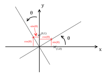
Therefore the matrix $\mathbf{A}$ that represents this transformation satisfies
$$ \begin{align} \mathbf{AI} &= \left( \begin{array}{cc} \cos\theta & -\sin\theta \\ \sin\theta & \cos\theta \end{array} \right) \\ \Rightarrow \mathbf{A} &= \left( \begin{array}{cc} \cos\theta & -\sin\theta \\ \sin\theta & \cos\theta \end{array} \right) ~ \blacksquare \end{align} $$
Reflections
In FP1 you need to know the matrices that reflect objects (i) across the $y$-axis, (ii) across the $x$-axis, (iii) across $y=x$, and (iv) across $y=-x$.
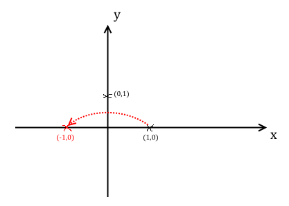
The matrix that reflects objects across the $y$-axis is $\left( \begin{array}{cc} -1 & 0 \\ 0 & 1 \end{array} \right)$.
The points forming $\mathbf{I}$ are flipped across the $y$-axis, changing $(1,0)$ to $(-1,0)$ and leaving $(0,1)$ unchanged.
The matrix that reflects objects across the $x$-axis is $\left( \begin{array}{cc} 1 & 0 \\ 0 & -1 \end{array} \right)$.
Reasoning similar to the reflection across the $y$-axis.
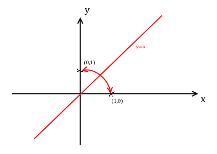
The matrix that reflects objects across the line $y=x$ is $\left( \begin{array}{cc} 0 & 1 \\ 1 & 0 \end{array} \right)$.
The points forming $\mathbf{I}$ are flipped across the line $y=x$. They are swapped with each other.
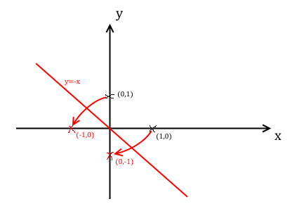
The matrix that reflects objects across the line $y=-x$ is $\left( \begin{array}{cc} 0 & -1 \\ -1 & 0 \end{array} \right)$.
The points $(1,0)$ and $(0,1)$ forming $\mathbf{I}$ are flipped across the line $y=-x$, and they are transformed to $(0,-1)$ and $(-1,0)$ respectively.
Enlargement
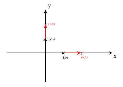
The matrix that enlarges an object by a scale factor $k$ with centre $(0,0)$ is $\left( \begin{array}{cc} k & 0 \\ 0 & k \end{array} \right)$.
Scale the points $(1,0)$ and $(0,1)$ forming $\mathbf{I}$ by scale factor $k$ with centre $(0,0)$ and they are transformed to $(k,0)$ and $(0,k)$ respectively.
You can also make the argument that $k\mathbf{I} = \left( \begin{array}{cc} k & 0 \\ 0 & k \end{array} \right)$.
Bear in mind that $k$ can be positive as well as negative.
Inverse transformations
If a non-singular matrix $\mathbf{A}$ represents a linear transformation, then $\mathbf{A}^{-1}$ undoes the transformation.
Let $\mathbf{A}$ be a non-singular matrix representing a transformation. The result of applying the transformation $\mathbf{A}$ to the object $\mathbf{S}$ is $\mathbf{AS}$.
Applying the transformation $\mathbf{A}^{-1}$ to the resulting object gives $\mathbf{A}^{-1}\mathbf{AS} = \mathbf{IS} = \mathbf{S} ~ \blacksquare$
Additional worked examples
Coming soon.